Step 3 — MPI Scalability (Amdahl/Gustafson)
1. Scope and cluster architecture
The objective was to deploy OpenMPI on the Raspberry Pi cluster, validate multi-node execution, measure strong and weak scaling, and use two MPI applications to demonstrate Amdahl's Law and Gustafson's Law.
| Role | Hardware / identity | Function |
|---|---|---|
| Master | Raspberry Pi 5, server-pi5 |
Runs mpirun and stores the shared worker root filesystem |
| Workers | 8 × Raspberry Pi 3 | Run all MPI application ranks |
| Worker IPs | 192.168.10.101–108 |
Static addresses used by SSH and the OpenMPI hostfile |
| Worker user | server-pi3 |
Common SSH and MPI execution account |
| Worker rootfs | /nfs/rootfs |
Single 64-bit PXE/NFS root filesystem shared by all workers |
| MPI capacity | 8 nodes × 4 cores | 32 ranks without oversubscription |
and PXE/NFS server
rpi3-node5 192.168.10.105 · rpi3-node6 192.168.10.106 · rpi3-node7 192.168.10.107 · rpi3-node8 192.168.10.108
All workers use the same 64-bit operating system and the shared root filesystem at /nfs/rootfs.
Rank placement: the Pi 5 launches the job but is not included in the worker hostfile. Therefore, all ranks—including rank 0—run on the homogeneous Pi 3 worker pool.
2. Final design decisions
Master used only as launcher
mpirun executes on server-pi5. The Pi 5 is excluded from MPI_COMM_WORLD, so the performance measurements compare identical Pi 3 nodes.
Shared worker environment
OpenMPI, programs, SSH configuration and benchmark files are installed once in the shared PXE/NFS environment and are consequently visible to all eight workers.
SSH-based OpenMPI launch
Passwordless SSH works from the master to every worker and between workers. The worker account is always server-pi3.
Homogeneous compilation target
The applications are built on the Pi 5 for the Pi 3 worker CPU using -mcpu=cortex-a53, avoiding Pi-5-specific native optimizations.
3. Step-by-step replication procedure
Unless a step explicitly says otherwise, run commands on server-pi5. Use a normal non-root user to launch MPI jobs.
-
Confirm the workers are reachable
-
Define stable worker names
Add the following entries to both /etc/hosts on the master and /nfs/rootfs/etc/hosts for the workers:
192.168.10.101    rpi3-node1
192.168.10.102    rpi3-node2
192.168.10.103    rpi3-node3
192.168.10.104    rpi3-node4
192.168.10.105    rpi3-node5
192.168.10.106    rpi3-node6
192.168.10.107    rpi3-node7
192.168.10.108    rpi3-node8
-
Install OpenMPI on the master
-
Install OpenMPI once in the shared worker root filesystem
Inside the chroot:
apt update
apt install -y           openmpi-bin           libopenmpi-dev           build-essential           openssh-server           openssh-client           time           bc           python3

mpirun --version
mpicc --version
exit
Back on the master:
sudo umount /nfs/rootfs/run
sudo umount /nfs/rootfs/sys
sudo umount /nfs/rootfs/proc
sudo umount /nfs/rootfs/dev
-
Create one shared MPI project path
The same absolute application path must exist on the launcher and workers. The worker view of /nfs/rootfs/srv/mpi is /srv/mpi, so it is bind-mounted at the same path on the master.
sudo mkdir -p /nfs/rootfs/srv/mpi
sudo mkdir -p /srv/mpi
sudo mount --bind /nfs/rootfs/srv/mpi /srv/mpi

echo "/nfs/rootfs/srv/mpi /srv/mpi none bind 0 0"           | sudo tee -a /etc/fstab

sudo mkdir -p /srv/mpi/{src,bin,hosts,results}
sudo chown -R "$USER":"$USER" /srv/mpi
-
Configure passwordless master-to-worker SSH
The public key used by the master must be accepted by the shared worker account. Since the worker home is shared, adding it once makes it available on all workers.
mkdir -p ~/.ssh
chmod 700 ~/.ssh

# Generate this key only if the master does not already have one.
test -f ~/.ssh/id_ed25519 || ssh-keygen -t ed25519 -N "" -f ~/.ssh/id_ed25519

ssh-copy-id server-pi3@192.168.10.101
Use the following master-side SSH configuration in ~/.ssh/config:
Host 192.168.10.101 192.168.10.102 192.168.10.103 192.168.10.104 192.168.10.105 192.168.10.106 192.168.10.107 192.168.10.108
  User server-pi3
  BatchMode yes
  ConnectTimeout 5
  StrictHostKeyChecking accept-new
chmod 600 ~/.ssh/config

for ip in 192.168.10.{101..108}; do
    ssh -o BatchMode=yes "$ip" hostname
done
-
Configure worker-to-worker passwordless SSH
Log in to one worker and create a dedicated cluster key. Because /home/server-pi3 is shared through the worker root filesystem, the same key and authorization are immediately available on every worker.
ssh server-pi3@192.168.10.101

mkdir -p ~/.ssh
chmod 700 ~/.ssh

ssh-keygen -t ed25519 -f ~/.ssh/id_ed25519_mpi -N "" -C "server-pi3 MPI worker key"

touch ~/.ssh/authorized_keys
grep -qxF "$(cat ~/.ssh/id_ed25519_mpi.pub)"           ~/.ssh/authorized_keys ||           cat ~/.ssh/id_ed25519_mpi.pub >> ~/.ssh/authorized_keys

chmod 600 ~/.ssh/authorized_keys
chmod 600 ~/.ssh/id_ed25519_mpi
chmod 644 ~/.ssh/id_ed25519_mpi.pub
Place the following in the shared worker ~/.ssh/config:
Host 192.168.10.101 192.168.10.102 192.168.10.103 192.168.10.104 192.168.10.105 192.168.10.106 192.168.10.107 192.168.10.108
  User server-pi3
  IdentityFile ~/.ssh/id_ed25519_mpi
  IdentitiesOnly yes
  BatchMode yes
  ConnectTimeout 5
  StrictHostKeyChecking accept-new
chmod 600 ~/.ssh/config
touch ~/.ssh/known_hosts
chmod 600 ~/.ssh/known_hosts

for ip in 192.168.10.{101..108}; do
    ssh-keyscan -H "$ip" >> ~/.ssh/known_hosts 2>/dev/null
done

sort -u ~/.ssh/known_hosts -o ~/.ssh/known_hosts

for ip in 192.168.10.{101..108}; do
    ssh -o BatchMode=yes "$ip" hostname
done

exit
-
Create the OpenMPI
hostfile
Save the following as /srv/mpi/hosts/pi3.hosts:
192.168.10.101 slots=4 max_slots=4
192.168.10.102 slots=4 max_slots=4
192.168.10.103 slots=4 max_slots=4
192.168.10.104 slots=4 max_slots=4
192.168.10.105 slots=4 max_slots=4
192.168.10.106 slots=4 max_slots=4
192.168.10.107 slots=4 max_slots=4
192.168.10.108 slots=4 max_slots=4
This exposes four slots per Pi 3 and a total of 32 ranks without oversubscription.
-
Compile and validate the MPI hello program
Save the hello source shown in Appendix A as /srv/mpi/src/hello.c, then run:
mpicc -O2 -mcpu=cortex-a53 -o /srv/mpi/bin/hello /srv/mpi/src/hello.c

mpirun --hostfile /srv/mpi/hosts/pi3.hosts -np 32 --map-by node --bind-to core --tag-output /srv/mpi/bin/hello
With --map-by node, ranks are distributed round-robin. At 32 ranks each Pi 3 receives four ranks, while rank 0 runs on the first Pi 3—not on the Pi 5 launcher.
-
Compile the two benchmark applications
Save the sources from Appendix A as /srv/mpi/src/pi_reduce.c and /srv/mpi/src/stencil1d.c.
mpicc -O3 -mcpu=cortex-a53 -o /srv/mpi/bin/pi_reduce /srv/mpi/src/pi_reduce.c
mpicc -O3 -mcpu=cortex-a53 -o /srv/mpi/bin/stencil1d /srv/mpi/src/stencil1d.c
-
Install the rigorous benchmark and analysis scripts
Save the scripts from Appendix B as: /srv/mpi/run_benchmarks.sh and /srv/mpi/analyze_results.py.
chmod +x /srv/mpi/run_benchmarks.sh
chmod +x /srv/mpi/analyze_results.py

/srv/mpi/run_benchmarks.sh

python3 /srv/mpi/analyze_results.py
The successful run creates files under:
/srv/mpi/results/pi.csv
/srv/mpi/results/pi_summary.csv
/srv/mpi/results/pi_scaling_plots_mpi.png

/srv/mpi/results/stencil.csv
/srv/mpi/results/stencil_summary.csv
/srv/mpi/results/stencil_scaling_plots_mpi.png
4. MPI applications used in the evaluation
pi_reduce
The program approximates π by numerically integrating 4/(1+x²) over the interval 0 to 1. Integration points are divided among ranks in a cyclic pattern. Each rank computes a local partial sum, and MPI_Reduce adds the partial results on rank 0.
The main calculation is independent and requires almost no communication until the final reduction. It therefore represents a compute-dominated MPI workload.
stencil1d
The program repeatedly smooths a one-dimensional array using the update 0.25 × left + 0.50 × centre + 0.25 × right. The global array is split into contiguous rank-local sections.
Every iteration requires neighboring ranks to exchange boundary, or halo, values using MPI_Sendrecv. A final MPI_Allreduce produces a checksum. This represents a communication- and synchronization-sensitive workload.
Both applications include an explicit serial loop executed by rank 0. This gives the analysis a measurable serial component for illustrating Amdahl’s and Gustafson’s laws. Rank 0 still participates in the main parallel computation.
5. Benchmark methodology
The final measurements used the rigorous shell harness without changing its default parameters.
Rank counts
1, 2, 4, 8, 16 and 32 ranks.
Repetitions
Three runs for every case.
Statistic
The mean total time at each rank count.
Mapping
--map-by node distributes ranks round-robin.
Binding
--bind-to core pins ranks to CPU cores.
Capacity
--nooversubscribe enforces the 32-slot limit.
Default workloads
| Benchmark | Scaled workload |
|---|---|
| π | 100,000,000 200,000,000 400,000,000 800,000,000 1,600,000,000 3,200,000,000 (steps) |
| Stencil 1D | 1,000,000 2,000,000 4,000,000 8,000,000 (cells/rank) |
Metrics
Speedup: T₁ / Tₙ
Efficiency: speedup / n
6. Final measured results
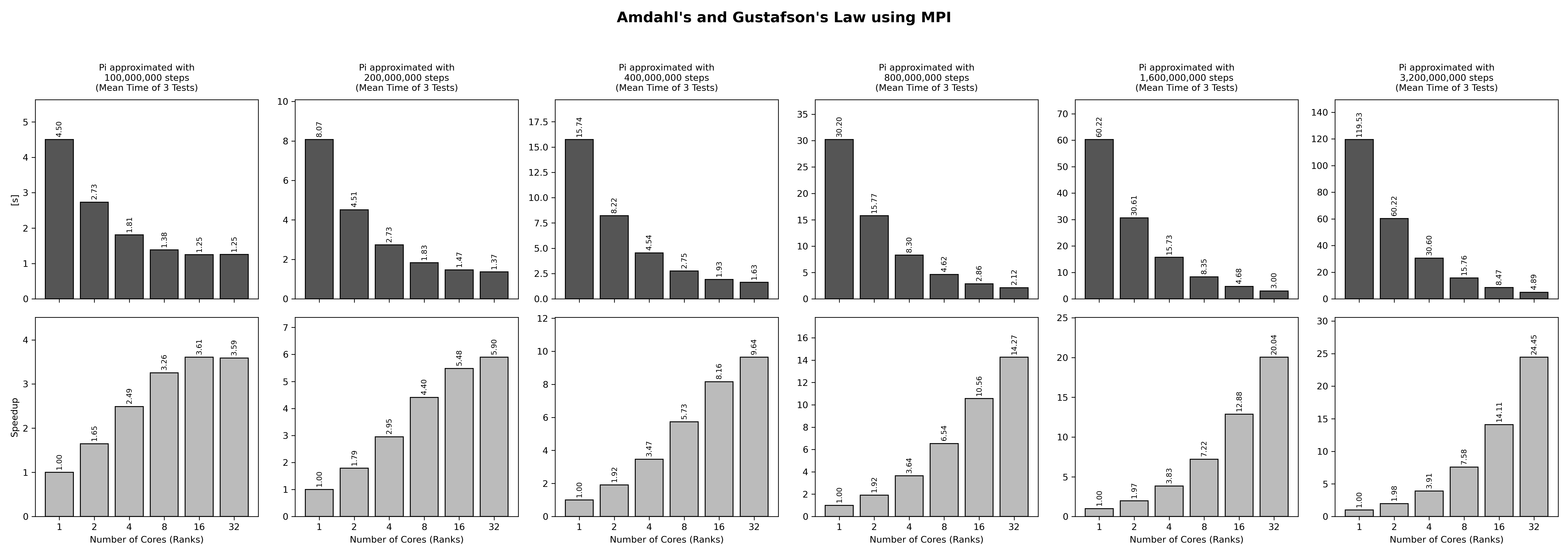
24.45× π speedup at 32 ranks
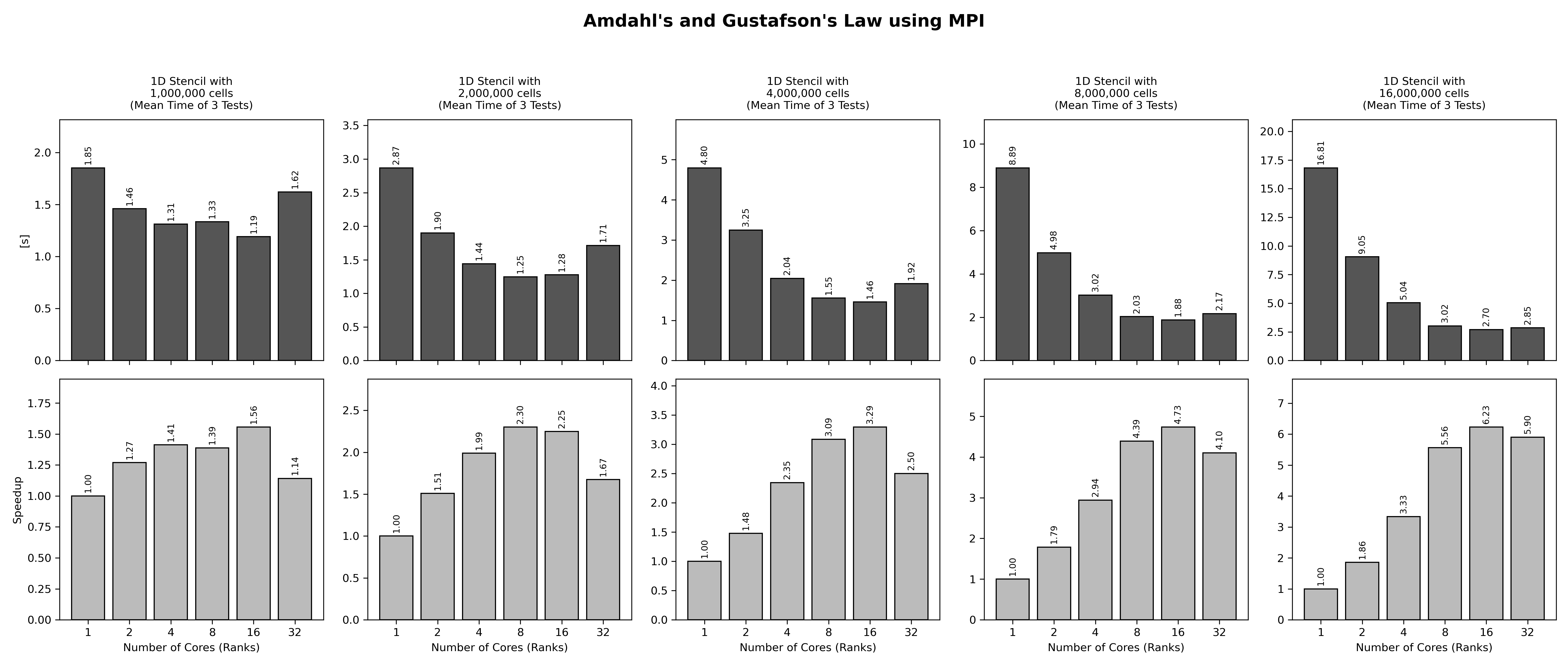
6.23x Stencil speedup at 16 ranks
π scaling
| Steps for calculation | Ranks | Runs | Average Time (s) | Speedup |
|---|---|---|---|---|
| 100,000,000 | 1 | 3 | 4.50 | 1.00 |
| 100,000,000 | 2 | 3 | 2.73 | 1.65 |
| 100,000,000 | 4 | 3 | 1.81 | 2.49 |
| 100,000,000 | 8 | 3 | 1.38 | 3.26 |
| 100,000,000 | 16 | 3 | 1.25 | 3.61 |
| 100,000,000 | 32 | 3 | 1.25 | 3.59 |
| 200,000,000 | 1 | 3 | 8.07 | 1.00 |
| 200,000,000 | 2 | 3 | 4.51 | 1.79 |
| 200,000,000 | 4 | 3 | 2.73 | 2.95 |
| 200,000,000 | 8 | 3 | 1.83 | 4.40 |
| 200,000,000 | 16 | 3 | 1.47 | 5.48 |
| 200,000,000 | 32 | 3 | 1.37 | 5.90 |
| 400,000,000 | 1 | 3 | 15.74 | 1.00 |
| 400,000,000 | 2 | 3 | 8.22 | 1.92 |
| 400,000,000 | 4 | 3 | 4.54 | 3.47 |
| 400,000,000 | 8 | 3 | 2.75 | 5.73 |
| 400,000,000 | 16 | 3 | 1.93 | 8.16 |
| 400,000,000 | 32 | 3 | 1.63 | 9.64 |
| 800,000,000 | 1 | 3 | 30.20 | 1.00 |
| 800,000,000 | 2 | 3 | 15.77 | 1.92 |
| 800,000,000 | 4 | 3 | 8.30 | 3.64 |
| 800,000,000 | 8 | 3 | 4.62 | 6.54 |
| 800,000,000 | 16 | 3 | 2.86 | 10.56 |
| 800,000,000 | 32 | 3 | 2.12 | 14.27 |
| 1,600,000,000 | 1 | 3 | 60.22 | 1.00 |
| 1,600,000,000 | 2 | 3 | 30.61 | 1.97 |
| 1,600,000,000 | 4 | 3 | 15.73 | 3.83 |
| 1,600,000,000 | 8 | 3 | 8.35 | 7.22 |
| 1,600,000,000 | 16 | 3 | 4.68 | 12.88 |
| 1,600,000,000 | 32 | 3 | 3.00 | 20.04 |
| 3,200,000,000 | 1 | 3 | 119.53 | 1.00 |
| 3,200,000,000 | 2 | 3 | 60.22 | 1.98 |
| 3,200,000,000 | 4 | 3 | 30.60 | 3.91 |
| 3,200,000,000 | 8 | 3 | 15.76 | 7.58 |
| 3,200,000,000 | 16 | 3 | 8.47 | 14.11 |
| 3,200,000,000 | 32 | 3 | 4.89 | 24.45 |
Stencil scaling
| Total Cells | Ranks | Runs | Average Time (s) | Speedup |
|---|---|---|---|---|
| 1,000,000 | 1 | 3 | 1.85 | 1.00 |
| 1,000,000 | 2 | 3 | 1.46 | 1.27 |
| 1,000,000 | 4 | 3 | 1.31 | 1.41 |
| 1,000,000 | 8 | 3 | 1.33 | 1.39 |
| 1,000,000 | 16 | 3 | 1.19 | 1.56 |
| 1,000,000 | 32 | 3 | 1.62 | 1.14 |
| 2,000,000 | 1 | 3 | 2.87 | 1.00 |
| 2,000,000 | 2 | 3 | 1.90 | 1.51 |
| 2,000,000 | 4 | 3 | 1.44 | 1.99 |
| 2,000,000 | 8 | 3 | 1.25 | 2.30 |
| 2,000,000 | 16 | 3 | 1.28 | 2.25 |
| 2,000,000 | 32 | 3 | 1.71 | 1.67 |
| 4,000,000 | 1 | 3 | 4.80 | 1.00 |
| 4,000,000 | 2 | 3 | 3.25 | 1.48 |
| 4,000,000 | 4 | 3 | 2.04 | 2.35 |
| 4,000,000 | 8 | 3 | 1.55 | 3.09 |
| 4,000,000 | 16 | 3 | 1.46 | 3.29 |
| 4,000,000 | 32 | 3 | 1.92 | 2.50 |
| 8,000,000 | 1 | 3 | 8.89 | 1.00 |
| 8,000,000 | 2 | 3 | 4.98 | 1.78 |
| 8,000,000 | 4 | 3 | 3.02 | 2.94 |
| 8,000,000 | 8 | 3 | 2.03 | 4.39 |
| 8,000,000 | 16 | 3 | 1.88 | 4.73 |
| 8,000,000 | 32 | 3 | 2.17 | 4.10 |
| 16,000,000 | 1 | 3 | 16.81 | 1.00 |
| 16,000,000 | 2 | 3 | 9.05 | 1.86 |
| 16,000,000 | 4 | 3 | 5.04 | 3.33 |
| 16,000,000 | 8 | 3 | 3.02 | 5.56 |
| 16,000,000 | 16 | 3 | 2.70 | 6.23 |
| 16,000,000 | 32 | 3 | 2.85 | 5.90 |
7. Amdahl's Law and Gustafson's Law
8. Interpretation of the results
8.1 π scaling
The Pi calculation clearly demonstrate Amdahl's Law. As the number of cores increases for a fixed problem size, the execution time drops sharply, pushing the maximum speedup to 24.45× on the largest workload. However, the charts also reveal Amdahl's limitation: for smaller problem sizes, the speedup flattens out early around 3.59×. This happens because the math finishes so quickly that fixed communication and synchronization overheads begin to dominate the run time. When the problem size is scaled up, the computation outpaces this overhead, allowing the system to achieve much better parallel efficiency.
8.2 stencil scaling
The results provide an excellent representation of Amdahl's Law. As the total number of cells remains fixed for each graph, adding more processing cores successfully reduces the execution time, with the largest workload dropping from 16.81 seconds down to 2.85 seconds. This trend yields a clear upward climb in speedup, reaching a peak efficiency of 6.23× at 16 ranks on the largest dataset. However, the 32-rank mark reveals a physical limitation where performance slightly regresses across all test groups. This drop-off occurs because dividing a fixed workload across 32 ranks reduces the local math per core so much that the overhead of network communication between the 8 Raspberry Pi boards becomes the dominant bottleneck.
8.3 Why 32 ranks provide less speedup than 16 ranks
With 16 ranks and --map-by node, the system places two ranks at each of the 8 nodes; at 32 ranks, every node hosts four.
Above eight ranks, multiple MPI processes share each Pi’s processor caches, memory system and network interface. The affects stencil streams more than π through large arrays and repeatedly exchanging halo data with neighboring ranks, whereas π performs mostly independent arithmetic and communicates primarily at the end.
9. Conclusion
The OpenMPI deployment successfully converted the eight Raspberry Pi 3 workers into a 32-rank compute pool controlled by the Raspberry Pi 5 launcher.
- The shared
PXE/NFSroot filesystem allowed OpenMPI and the benchmark applications to be installed once for all workers. - Passwordless master-to-worker and worker-to-worker SSH enabled reliable multi-node launch.
- The Pi 5 remained outside the measured MPI communicator, preserving a homogeneous Pi 3 performance baseline.
- The compute-dominated π program achieved 24.45× speedup.
- The communication-sensitive stencil achieved its best fixed-size runtime for maximum problem size at 16 ranks and showed relatively less throughput gain when increasing from 16 to 32 ranks.
- Amdahl’s Law was demonstrated by diminishing fixed-size speedup, while Gustafson’s Law was demonstrated most clearly by the nearly constant runtime of the scaled π workload.
Final assessment: the cluster is effective for parallel workloads with a high computation-to-communication ratio. Communication-intensive workloads benefit up to the point where inter-rank messaging and shared per-node resources dominate the useful work.
10. Complete source files and scripts
The appendices below make the document self-contained. Each listing can be copied directly to the path stated in the replication procedure.
Appendix A: MPI application sources
/srv/mpi/src/hello.c
#include <mpi.h>
#include <stdio.h>
#include <unistd.h>

int main(int argc, char **argv) {
    MPI_Init(&argc, &argv);

    int rank, size;
    char host[256];

    MPI_Comm_rank(MPI_COMM_WORLD, &rank);
    MPI_Comm_size(MPI_COMM_WORLD, &size);
    gethostname(host, sizeof(host));

    printf("Hello from rank %d of %d on %s\n", rank, size, host);

    MPI_Finalize();
    return 0;
}
/srv/mpi/src/pi_reduce.c
#include <mpi.h>
#include <stdio.h>
#include <stdlib.h>

int main(int argc, char **argv) {
    MPI_Init(&argc, &argv);

    int rank, size;
    MPI_Comm_rank(MPI_COMM_WORLD, &rank);
    MPI_Comm_size(MPI_COMM_WORLD, &size);

    unsigned long long steps = 50000000ULL;
    unsigned long long serial_iters = 0ULL;

    if (argc >= 2) steps = strtoull(argv[1], NULL, 10);
    if (argc >= 3) serial_iters = strtoull(argv[2], NULL, 10);

    MPI_Barrier(MPI_COMM_WORLD);
    double t0 = MPI_Wtime();

    double serial_value = 0.0;
    double serial_time = 0.0;

    MPI_Bcast(&serial_value, 1, MPI_DOUBLE, 0, MPI_COMM_WORLD);
    MPI_Bcast(&serial_time, 1, MPI_DOUBLE, 0, MPI_COMM_WORLD);

    MPI_Barrier(MPI_COMM_WORLD);
    double tp0 = MPI_Wtime();

    double step = 1.0 / (double)steps;
    double local_sum = 0.0;

    for (unsigned long long i = (unsigned long long)rank;
         i < steps;
         i += (unsigned long long)size) {
        double x = ((double)i + 0.5) * step;
        local_sum += 4.0 / (1.0 + x * x);
    }

    double local_pi = local_sum * step;
    double pi = 0.0;

    MPI_Reduce(&local_pi, &pi, 1, MPI_DOUBLE,
               MPI_SUM, 0, MPI_COMM_WORLD);

    MPI_Barrier(MPI_COMM_WORLD);
    double t1 = MPI_Wtime();

    if (rank == 0) {
        double parallel_time = t1 - tp0;
        double total_time = t1 - t0;
        printf("pi_reduce,%d,%llu,%llu,%.9f,%.9f,%.9f,%.15f\n",
               size, steps, serial_iters, serial_time,
               parallel_time, total_time, pi);
    }

    MPI_Finalize();
    return 0;
}
/srv/mpi/src/stencil1d.c
#include <mpi.h>
#include <stdio.h>
#include <stdlib.h>

int main(int argc, char **argv) {
    MPI_Init(&argc, &argv);

    int rank, size;
    MPI_Comm_rank(MPI_COMM_WORLD, &rank);
    MPI_Comm_size(MPI_COMM_WORLD, &size);

    long long total_cells = 4000000LL;
    int iterations = 100;
    unsigned long long serial_iters = 0ULL;

    if (argc >= 2) total_cells = atoll(argv[1]);
    if (argc >= 3) iterations = atoi(argv[2]);
    if (argc >= 4) serial_iters = strtoull(argv[3], NULL, 10);

    long long base = total_cells / size;
    long long rem = total_cells % size;
    long long n = base + (rank < rem ? 1 : 0);

    if (n < 1) {
        if (rank == 0) {
            fprintf(stderr,
                    "total_cells must be >= number of ranks\n");
        }
        MPI_Abort(MPI_COMM_WORLD, 1);
    }

    double *a = calloc((size_t)n + 2, sizeof(double));
    double *b = calloc((size_t)n + 2, sizeof(double));

    if (!a || !b) {
        fprintf(stderr,
                "rank %d: allocation failed for %lld cells\n",
                rank, n);
        MPI_Abort(MPI_COMM_WORLD, 2);
    }

    for (long long i = 1; i <= n; i++) {
        a[i] = 0.001 * (double)(rank + 1)
             + 0.000001 * (double)(i % 1000);
    }

    MPI_Barrier(MPI_COMM_WORLD);
    double t0 = MPI_Wtime();

    double serial_value = 0.0;
    double serial_time = 0.0;

    MPI_Bcast(&serial_value, 1, MPI_DOUBLE, 0, MPI_COMM_WORLD);
    MPI_Bcast(&serial_time, 1, MPI_DOUBLE, 0, MPI_COMM_WORLD);

    int left = rank - 1;
    int right = rank + 1;
    if (left < 0) left = MPI_PROC_NULL;
    if (right >= size) right = MPI_PROC_NULL;

    double comm_time = 0.0;
    double compute_time = 0.0;

    for (int it = 0; it < iterations; it++) {
        double tc0 = MPI_Wtime();

        MPI_Sendrecv(&a[1], 1, MPI_DOUBLE, left, 10,
                     &a[n + 1], 1, MPI_DOUBLE, right, 10,
                     MPI_COMM_WORLD, MPI_STATUS_IGNORE);

        MPI_Sendrecv(&a[n], 1, MPI_DOUBLE, right, 20,
                     &a[0], 1, MPI_DOUBLE, left, 20,
                     MPI_COMM_WORLD, MPI_STATUS_IGNORE);

        if (left == MPI_PROC_NULL) a[0] = a[1];
        if (right == MPI_PROC_NULL) a[n + 1] = a[n];

        comm_time += MPI_Wtime() - tc0;

        double tw0 = MPI_Wtime();

        for (long long i = 1; i <= n; i++) {
            b[i] = 0.25 * a[i - 1]
                 + 0.50 * a[i]
                 + 0.25 * a[i + 1];
        }

        double *tmp = a;
        a = b;
        b = tmp;

        compute_time += MPI_Wtime() - tw0;
    }

    double local_sum = 0.0;
    for (long long i = 1; i <= n; i++) {
        local_sum += a[i];
    }

    double checksum = 0.0;
    MPI_Allreduce(&local_sum, &checksum, 1, MPI_DOUBLE,
                  MPI_SUM, MPI_COMM_WORLD);

    double max_comm_time = 0.0;
    double max_compute_time = 0.0;

    MPI_Reduce(&comm_time, &max_comm_time, 1, MPI_DOUBLE,
               MPI_MAX, 0, MPI_COMM_WORLD);
    MPI_Reduce(&compute_time, &max_compute_time, 1, MPI_DOUBLE,
               MPI_MAX, 0, MPI_COMM_WORLD);

    MPI_Barrier(MPI_COMM_WORLD);
    double t1 = MPI_Wtime();

    if (rank == 0) {
        double total_time = t1 - t0;
        printf("stencil1d,%d,%lld,%d,%llu,"
               "%.9f,%.9f,%.9f,%.9f,%.12f\n",
               size, total_cells, iterations, serial_iters,
               serial_time, max_comm_time, max_compute_time,
               total_time, checksum);
    }

    free(a);
    free(b);

    MPI_Finalize();
    return 0;
}
Appendix B: Benchmark and analysis scripts
/srv/mpi/run_benchmarks.sh
#!/bin/bash

# Output CSV files
PI_CSV="/srv/mpi/results/pi.csv"
STENCIL_CSV="/srv/mpi/results/stencil.csv"

# Number of iterations for robust data
NUM_RUNS=3


HOST_FILE="/srv/mpi/hosts/pi3.hosts"
PI_PROGRAM="/srv/mpi/bin/pi_reduce"
STENCIL_PROGRAM="/srv/mpi/bin/stencil1d"

echo "problem_size,ranks,run,execution_time" > "$PI_CSV"
echo "cells_per_rank,ranks,run,execution_time" > "$STENCIL_CSV"

RANKS_SETS=(1 2 4 8 16 32)
PI_SIZES=(100000000 200000000 400000000 800000000 1600000000 3200000000)
STENCIL_SIZES=(1000000 2000000 4000000 8000000 16000000)
ITERATIONS=100

[ -f "$PI_PROGRAM" ] && chmod +x "$PI_PROGRAM"
[ -f "$STENCIL_PROGRAM" ] && chmod +x "$STENCIL_PROGRAM"

# Sanity Check
if [ ! -x "$PI_PROGRAM" ] || [ ! -x "$STENCIL_PROGRAM" ]; then
    echo "ERROR: Binaries not found or not executable in $CURRENT_DIR"
    echo "Expected files: 'pi_reduce' and 'stencil1d'"
    echo "Please ensure you have compiled them here first."
    exit 1
fi

echo "=== Starting Pi Calculation Benchmarks ==="
for size in "${PI_SIZES[@]}"; do
    echo "Running problem size: $size steps"
    for ranks in "${RANKS_SETS[@]}"; do
        for run in $(seq 1 $NUM_RUNS); do
            echo "  -> Ranks: $ranks | Run: $run"
            START_TIME=$(date +%s.%N)
            OUTPUT=$(mpirun --hostfile "$HOST_FILE" -np "$ranks" --map-by node --bind-to core --tag-output "$PI_PROGRAM" "$size" 0)
            END_TIME=$(date +%s.%N)

            ELAPSED=$(echo "$END_TIME - $START_TIME" | bc)

            echo "$size,$ranks,$run,$ELAPSED" >> "$PI_CSV"
        done
    done
done

echo "=== Starting Stencil 1D Benchmarks ==="
for cells in "${STENCIL_SIZES[@]}"; do
    echo "Running $cells cells per rank"
    for ranks in "${RANKS_SETS[@]}"; do
        for run in $(seq 1 $NUM_RUNS); do
            echo "  -> Ranks: $ranks | Run: $run"
            # Gustafson's Law: total cells = cells_per_rank * ranks
            TOTAL_CELLS=$(( cells ))

            START_TIME=$(date +%s.%N)
            OUTPUT=$(mpirun -np "$ranks" --map-by node --bind-to core --tag-output "$STENCIL_PROGRAM" "$TOTAL_CELLS" "$ITERATIONS" 0)
            END_TIME=$(date +%s.%N)

            ELAPSED=$(echo "$END_TIME - $START_TIME" | bc)

            echo "$cells,$ranks,$run,$ELAPSED" >> "$STENCIL_CSV"
        done
    done
done

echo "=== Benchmarks Completed! ==="
echo "Results saved to $PI_CSV and $STENCIL_CSV"
/srv/mpi/analyze_results.py
#!/usr/bin/env python3
import pandas as pd
import matplotlib.pyplot as plt
import numpy as np

def process_and_plot(csv_file, output_summary_csv, output_plot_img, main_title, title_template, is_stencil=False):
    # Load raw data
    df = pd.read_csv(csv_file)

    # 1. Calculate average execution time per configuration
    group_col = 'cells_per_rank' if is_stencil else 'problem_size'
    summary = df.groupby([group_col, 'ranks'])['execution_time'].mean().reset_index()
    summary = summary.rename(columns={'execution_time': 'avg_execution_time'})

    # 2. Calculate speedup: T_1 / T_p
    rank1_times = summary[summary['ranks'] == 1].set_index(group_col)['avg_execution_time'].to_dict()

    def calc_speedup(row):
        t1 = rank1_times.get(row[group_col])
        if t1 is None:
            return np.nan
        return t1 / row['avg_execution_time']

    summary['speedup'] = summary.apply(calc_speedup, axis=1)

    # Save the aggregated results to a new CSV file
    summary_to_save = summary.copy()
    summary_to_save['avg_execution_time'] = summary_to_save['avg_execution_time'].round(2)
    summary_to_save['speedup'] = summary_to_save['speedup'].round(2)
    summary_to_save.to_csv(output_summary_csv, index=False)
    print(f"Saved summary to {output_summary_csv}")

    # 3. Replicate the graph grid from image_5915db.jpg
    unique_sizes = sorted(summary[group_col].unique())
    num_cols = len(unique_sizes)

    # Create a 2xN grid layout
    fig, axes = plt.subplots(2, num_cols, figsize=(4 * num_cols, 8.5), sharex='col')

    # --- ADD MAIN HEADING HERE ---
    fig.suptitle(main_title, fontsize=16, fontweight='bold', y=0.98)

    for idx, size in enumerate(unique_sizes):
        sub_df = summary[summary[group_col] == size].sort_values('ranks')

        ranks_str = [str(r) for r in sub_df['ranks']]
        times = sub_df['avg_execution_time'].values
        speedups = sub_df['speedup'].values

        # --- Top Row: Average Execution Time ---
        ax_time = axes[0, idx]
        bars_time = ax_time.bar(ranks_str, times, color='#555555', edgecolor='black', width=0.8)
        ax_time.set_ylabel('[s]' if idx == 0 else '')

        formatted_size = f"{size:,}"
        ax_time.set_title(title_template.format(formatted_size), fontsize=10, pad=10)

        for bar in bars_time:
            height = bar.get_height()
            ax_time.annotate(f'{height:.2f}',
                             xy=(bar.get_x() + bar.get_width() / 2, height),
                             xytext=(0, 3),
                             textcoords="offset points",
                             ha='center', va='bottom', fontsize=8, rotation=90)

        ax_time.set_ylim(0, max(times) * 1.25)
        ax_time.tick_params(axis='both', which='both', length=4)

        # --- Bottom Row: Speedup ---
        ax_speed = axes[1, idx]
        bars_speed = ax_speed.bar(ranks_str, speedups, color='#bbbbbb', edgecolor='black', width=0.8)
        ax_speed.set_ylabel('Speedup' if idx == 0 else '')
        ax_speed.set_xlabel('Number of Cores (Ranks)')

        for bar in bars_speed:
            height = bar.get_height()
            ax_speed.annotate(f'{height:.2f}',
                             xy=(bar.get_x() + bar.get_width() / 2, height),
                             xytext=(0, 3),
                             textcoords="offset points",
                             ha='center', va='bottom', fontsize=8, rotation=90)

        ax_speed.set_ylim(0, max(speedups) * 1.25)
        ax_speed.tick_params(axis='both', which='both', length=4)

    # Adjust tight_layout to make sure it doesn't collide with the suptitle
    plt.tight_layout(rect=[0, 0, 1, 0.95])
    plt.savefig(output_plot_img, dpi=300)
    plt.close()
    print(f"Saved plot matrix to {output_plot_img}")

# Run for Pi (Amdahl's law)
process_and_plot(
    csv_file='/srv/mpi/results/pi.csv',
    output_summary_csv='/srv/mpi/results/pi_summary.csv',
    output_plot_img='/srv/mpi/results/pi_scaling_plots_mpi.png',
    main_title="Amdahl's and Gustafson's Law using MPI",
    title_template="Pi approximated with\n{} steps\n(Mean Time of 3 Tests)",
    is_stencil=False
)

# Run for Stencil 1D (Gustafson's law)
process_and_plot(
    csv_file='/srv/mpi/results/stencil.csv',
    output_summary_csv='/srv/mpi/results/stencil_summary.csv',
    output_plot_img='/srv/mpi/results/stencil_scaling_plots_mpi.png',
    main_title="Amdahl's and Gustafson's Law using MPI",
    title_template="1D Stencil with\n{} cells\n(Mean Time of 3 Tests)",
    is_stencil=True
)
Appendix C: Final hostfile
/srv/mpi/hosts/pi3.hosts