Cluster Performance Benchmark with HPL (High-Performance LINPACK)

A reproducible study of the floating-point performance (GFLOPS) and strong-scaling behaviour of a distributed edge computing cluster built from one Raspberry Pi 5 master and eight Raspberry Pi 3 worker nodes booted from a shared PXE/NFS root filesystem.

Master node Pi 5, hostname server-pi5 Workers 8 × Pi 3 nodes Benchmark HPL 2.3 (Netlib) Peak result 11.81 GFLOPS (8 workers, N=18000)

1. Scope and assumptions

This document records the procedure used to benchmark the cluster with HPL and the floating-point performance it achieved. HPL is the industry-standard implementation of the LINPACK benchmark: it solves a dense system of linear equations in double precision and reports the sustained rate of execution in GFLOPS, together with a residual check that verifies the computed solution is numerically correct.

• The Raspberry Pi 5 is used as the master/launcher only; it is not a compute node in these results.
• The eight Raspberry Pi 3 nodes are the compute workers.
• All Pi 3 workers boot from the Pi 5 via PXE/network boot and share one root filesystem at /nfs/rootfs.
• The worker login user is server-pi3; the master cluster IP is 192.168.10.1; workers are 192.168.10.101–108.
• A result is valid only when HPL reports PASSED on the residual check. A run that completes but reports FAILED is numerically wrong and its GFLOPS figure is meaningless.

Note

A large part of this task was diagnostic. Several non-obvious failure modes (architecture mismatch, a hard-coded BLAS path, the OpenMPI 5 transport layer, and a multi-rank-per-node corruption bug) had to be resolved before any multi-node run passed. The fixes are documented inline because they are the reproducibility-critical part of this task.

2. Cluster topology

Pi 5 master: server-pi5, 192.168.10.1
  ├── PXE/NFS rootfs for workers: /nfs/rootfs
  ├── HPL binary on master:        /opt/hpl/xhpl
  ├── HPL input file on master:    /opt/hpl/HPL.dat
  └── SSH access (as server-pi3) to 192.168.10.101 ... 108

Pi 3 workers (8 nodes, rpi3-node1 ... rpi3-node8):
  ├── Boot from shared PXE rootfs: /nfs/rootfs
  ├── HPL binary (shared via NFS): /opt/hpl/xhpl
  └── HPL input file (shared):     /opt/hpl/HPL.dat

The binary and the input file exist at the same path on the master and inside the shared rootfs, so every worker executes the identical xhpl and reads the identical HPL.dat. Both copies must be kept in sync whenever the configuration changes.

3. Software stack

Component	Version / package	Notes
HPL	2.3 (Netlib)	Compiled from source on a Pi 3.
MPI	OpenMPI 5.0.7	Identical version on master and all workers.
BLAS	OpenBLAS 0.3.29+ds-3	The serial variant (libopenblas0-serial); see §8.
Compiler	mpicc (GCC backend)	Target pinned to -mcpu=cortex-a53.
OS	64-bit Raspberry Pi OS / Debian trixie	Workers run from one shared aarch64 rootfs.

HPL uses the CBLAS interface (-DHPL_CALL_CBLAS), calling cblas_dgemm and friends in OpenBLAS.

4. Build HPL on a Pi 3 worker

HPL must be compiled for the worker CPU (Cortex-A53), not the master (Cortex-A76). Compiling on the Pi 5 with -march=native produces A76 instructions the A53 cannot execute, which crashed the workers. The reliable approach is to compile directly on a Pi 3 and pin the target architecture explicitly.

4.1 Key lines in Make.linux_arm

# BLAS interface: use the CBLAS interface
HPL_OPTS = -DHPL_CALL_CBLAS

# Linear algebra library: the SERIAL OpenBLAS build (see section 8)
LAdir = /usr/lib/aarch64-linux-gnu/openblas-serial
LAinc =
LAlib = -L$(LAdir) -lopenblas

# Compiler and flags: pin the CPU target explicitly to Cortex-A53
CC        = mpicc
CCFLAGS   = $(HPL_DEFS) -fomit-frame-pointer -O3 -funroll-loops -mcpu=cortex-a53
LINKER    = mpicc
LINKFLAGS = $(CCFLAGS)

Reproducibility note

The compiled xhpl has no rpath, so which physical OpenBLAS it loads at runtime is decided by the system-wide update-alternatives symlink, not by LAdir. Keep the whole BLAS alternatives family (libopenblas, libblas, liblapack) pointing at the same build; a mix of serial and pthread produces runtime symbol errors such as undefined symbol: sgemv_thread_n.

4.2 Compile

cd ~/hpl-2.3
make arch=linux_arm clean
make arch=linux_arm      # produces ~/hpl-2.3/bin/linux_arm/xhpl

5. Distribute the binary and HPL.dat

# from the master, copy the Pi 3-built binary to both locations
sudo scp -o "User=server-pi3" \
  rpi3-node1:/home/server-pi3/hpl-2.3/bin/linux_arm/xhpl /opt/hpl/xhpl
sudo chmod +x /opt/hpl/xhpl
sudo cp /opt/hpl/xhpl /nfs/rootfs/opt/hpl/xhpl

Note

The input file must be updated in both /opt/hpl/HPL.dat and /nfs/rootfs/opt/hpl/HPL.dat every time the configuration changes, or the master and workers will run different problems.

6. HPL.dat and the P×Q grid

A single HPL run is defined by three quantities: the matrix order N, the block size NB, and the process grid P×Q. The grid is how HPL knows how many workers to use and how to lay them out; P×Q must equal the number of MPI ranks. Because this cluster runs one rank per node (see §8), the grid also equals the number of worker nodes:

Workers	P × Q	Shape
1	1 × 1	single node
2	1 × 2	a row of two
4	2 × 2	square
8	2 × 4	two rows of four

Near-square grids communicate most efficiently, which is why these shapes are used. The block size was held at NB=192 throughout the study so that, within each problem size, the only variable is the worker count.

7. The mpirun invocation

mpirun --hostfile ~/hostfile_pi3_1rank -np 8 \
  --mca pml ob1 \
  --mca btl tcp,self \
  --mca btl_tcp_if_include eth0 \
  --mca pml_ucx_enabled 0 \
  --mca plm_rsh_args "-l server-pi3" \
  --map-by node \
  -x OMP_NUM_THREADS=1 -x OPENBLAS_NUM_THREADS=1 \
  --wdir /opt/hpl \
  /opt/hpl/xhpl

Flag	Why it is needed
--mca pml ob1 + pml_ucx_enabled 0	OpenMPI 5 defaults to the UCX transport, which is built for RDMA/InfiniBand and silently ignores the TCP settings. On this plain Ethernet switch UCX corrupted data and crashed. Forcing the ob1 layer and disabling UCX routes all traffic over plain TCP.
--mca btl tcp,self	Restricts byte transport to TCP and loopback; RDMA-oriented transports failed with "Socket closed" on this LAN.
--mca btl_tcp_if_include eth0	Pins MPI traffic to the wired interface.
--mca plm_rsh_args "-l server-pi3"	mpirun SSHes as the master user by default; the workers only accept the server-pi3 account.
--map-by node	Spreads ranks evenly across nodes.
-x OMP_NUM_THREADS=1 -x OPENBLAS_NUM_THREADS=1	One rank per core; all parallelism comes from MPI, so BLAS runs single-threaded.
--wdir /opt/hpl	Sets each rank's working directory to where HPL.dat lives, so every rank can open it.

8. Critical finding: one MPI rank per node

The single most important result for anyone replicating this work: on this cluster, running more than one MPI rank per Pi 3 node produced either a failed residual (numerically wrong answers) or a hard crash inside the OpenBLAS DGEMM kernel (dgemm_kernel_CORTEXA53). Running exactly one rank per node produced correct, verified results every time.

The following were each tested and ruled out as the cause:

• CPU architecture mismatch — eliminated by compiling on the Pi 3 with -mcpu=cortex-a53 and confirming an identical binary on every node.
• OpenBLAS thread oversubscription — eliminated by forcing single-threaded BLAS and by switching to the serial OpenBLAS build; the wrong answers persisted.
• Network / inter-node data exchange — eliminated because the failure reproduced with two ranks on a single node, with no network involved.
• A dead or unreachable node — eliminated; all eight nodes passed individually with one rank.

The decisive experiment: two ranks on one node failed, but one rank on each of two nodes PASSED. The common factor in every failure was multiple ranks sharing a single Pi 3's memory under OpenMPI 5 on the 64-bit shared NFS rootfs.

Practical consequence

The stable configuration uses one MPI rank per node with the serial OpenBLAS build. This is correct and verifiable, but it uses only one of each Pi 3's four cores, so the achieved GFLOPS is below the cluster's theoretical peak. An attempt to use all four cores per node via threaded OpenBLAS was unstable on the 1 GB nodes (it exhausted memory and lost worker daemons) and was set aside in favour of the correct, reproducible single-core-per-node result.

9. Benchmark methodology: the scaling sweep

To measure how performance scales with cluster size, HPL was run as a strong-scaling sweep: for each problem size N ∈ {5000, 8000, 18000}, the benchmark was run on 1, 2, 4 and 8 workers. Because HPL fixes the worker count at launch (via -np and the P×Q grid), each cell of this matrix is a separate invocation — it is not possible to sweep worker counts within a single HPL run.

Each cell was run five times and the reported GFLOPS is the mean of the five runs, matching the repeated-measurement methodology used elsewhere in this project. A cell that failed on its first attempt (see the memory wall in §11) was not repeated. In total the sweep comprised 50 runs. The block size was held at NB=192 throughout so that, within each problem size, worker count is the only variable.

The sweep was fully automated: a script regenerated HPL.dat (both copies) and the hostfile for each cell, launched the run with the flags from §7, parsed the GFLOPS / time / residual / pass-status from the output, and appended one row per run to a CSV. Run-to-run variation was small — the coefficient of variation stayed below 1.4% for every cell, and below 0.7% for most — indicating the measurements are stable and repeatable.

10. Results

All passing runs cleared the HPL residual check (scaled residual well under the 16.0 threshold). The figure below shows, for each problem size, the mean GFLOPS (top row) and the resulting speedup (bottom row) as the worker count increases. Error bars on the GFLOPS bars mark the min–max range across the five runs.

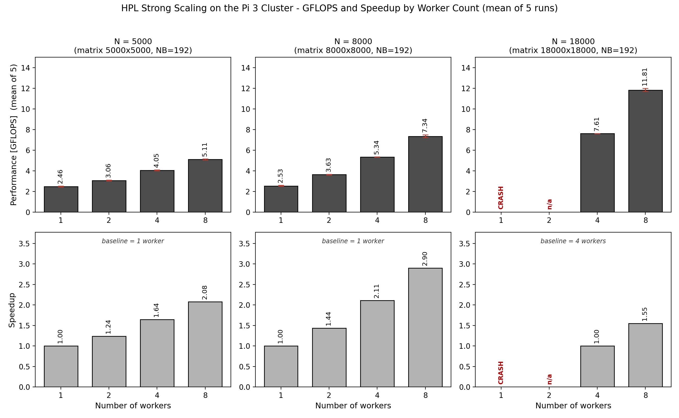HPL strong scaling on the Pi 3 cluster. Columns are fixed problem sizes; top row is mean GFLOPS (of 5 runs, min–max whiskers), bottom row is speedup vs the smallest working worker count. The N=18000 column has no 1- or 2-worker bar because the matrix does not fit in the memory of so few nodes (crash / out-of-memory), so its speedup is baselined at 4 workers.

10.1 Full result matrix (mean of 5 runs)

N	Workers	P×Q	Mean time [s]	Mean GFLOPS	Range [min–max]	Speedup	Status
5000	1	1×1	33.86	2.46	2.44–2.52	1.00	PASSED
5000	2	1×2	27.28	3.06	3.03–3.10	1.24	PASSED
5000	4	2×2	20.59	4.05	4.02–4.09	1.64	PASSED
5000	8	2×4	16.30	5.11	5.06–5.16	2.08	PASSED
8000	1	1×1	134.94	2.53	2.51–2.59	1.00	PASSED
8000	2	1×2	93.97	3.63	3.62–3.66	1.44	PASSED
8000	4	2×2	63.94	5.34	5.33–5.36	2.11	PASSED
8000	8	2×4	46.52	7.34	7.23–7.49	2.90	PASSED
18000	1	1×1	—	—	—	—	CRASH (OOM)
18000	2	1×2	—	—	—	—	OOM
18000	4	2×2	510.71	7.61	7.61–7.62	1.00 (base)	PASSED
18000	8	2×4	329.22	11.81	11.71–11.99	1.55	PASSED

Peak result: the eight-node cluster sustained 11.81 GFLOPS at N=18000 (2×4 grid), verified by the residual check (3.74×10⁻³).

11. Analysis and bottlenecks

11.1 Scaling improves with problem size

The speedup row shows the classic strong-scaling signature. At the smallest problem size the cluster scales poorly — N=5000 reaches only 2.08× on eight workers — because the matrix is small, each node finishes its share quickly, and inter-node communication (panel broadcasts and row/column swaps over TCP) consumes a large fraction of the run. As the problem grows there is more arithmetic to amortise that communication against, so scaling improves: N=8000 reaches 2.90× on eight workers, and N=18000 shows the strongest per-step scaling (1.55× from four to eight workers, against an ideal of 2×). This is a direct, measured illustration of the Amdahl / Gustafson principle that the benefit of parallelism depends on problem size.

11.2 The memory wall

An N=18000 matrix requires N²×8 bytes ≈ 2.6 GB, distributed across the workers. On a 1 GB Pi 3 this does not fit on one node (2.6 GB) or two nodes (1.3 GB each), which is exactly why those two cells crashed / ran out of memory. Only at four nodes (≈0.65 GB each) and eight nodes (≈0.32 GB each) does the problem fit. This is not a defect of the experiment but a measured demonstration of a real constraint: large problems require more nodes, both to go faster and simply to fit in memory.

11.3 Per-node efficiency and bottlenecks

Even where it scales, the cluster never reaches ideal speedup. Identified bottlenecks, roughly in order of impact:

• One core per node. The stability constraint of §8 caps the cluster at 8 of its 32 cores. Resolving multi-rank-per-node stability is the largest available performance gain.
• Interconnect. TCP-only transport on a consumer Ethernet switch adds latency to the communication that dominates HPL at small problem sizes; this is what flattens the N=5000 speedup curve.
• Memory. 1 GB per Pi 3 caps the problem size, which in turn limits the compute-to-communication ratio and therefore efficiency.
• Core microarchitecture. The in-order Cortex-A53 has modest double-precision throughput, setting a low per-core ceiling (~2.5 GFLOPS per node) regardless of tuning.

12. Conclusion and future work

Task 2 is complete: the cluster's floating-point performance was measured with HPL across a full strong-scaling sweep (three problem sizes × four worker counts, five repeats each) and verified by the residual check. The eight-node Pi 3 cluster reached a peak of 11.81 GFLOPS, and the sweep cleanly demonstrates that scaling efficiency rises with problem size while exposing a hard memory wall at N=18000 on few nodes. Alongside the numbers, the task produced a reproducible build procedure and documented several non-obvious failure modes — architecture mismatch, a hard-coded/mismatched BLAS path, the OpenMPI 5 UCX transport, and multi-rank-per-node memory corruption — each with its fix.

Two extensions would strengthen the result further:

• Use all 32 cores. Resolve the multi-rank-per-node instability — for example by testing MPICH in place of OpenMPI 5, or investigating the OpenMPI 5 shared-memory transport on the 64-bit NFS rootfs — to lift the cluster above its current one-core-per-node ceiling.
• Larger problem sizes on more nodes. With the memory wall mapped, deliberately choosing N to fill the aggregate RAM of the full eight-node cluster would push the sustained GFLOPS figure higher and further improve scaling efficiency.